

Since the discovery of the Higgs boson in 2012, scientists have been on an epic quest to measure its properties and hunt for any clues that might reveal new physics beyond the Standard Model (SM). One of the main studies consists of counting the number of Higgs bosons produced as a function of observables related to the Higgs boson itself, such as its transverse momentum, number of jets in the final state, etc. We call such studies differential measurements.
Several analysis groups have produced these measurements for the Higgs boson decaying in different ways: a pair of photons, two Z bosons, two W bosons and two tau leptons (both at high and low Higgs boson transverse momentum). CMS researchers have recently combined their measurements from Run 2 using sophisticated statistical techniques, with the goal of measuring these spectra in the most precise way and extracting the maximum amount of information from the data. An example of the combined measurement of the transverse momentum of the Higgs boson is shown in Figure 1. The measured values seem to agree with the SM predictions (the grey, green and red histograms), don’t you think?
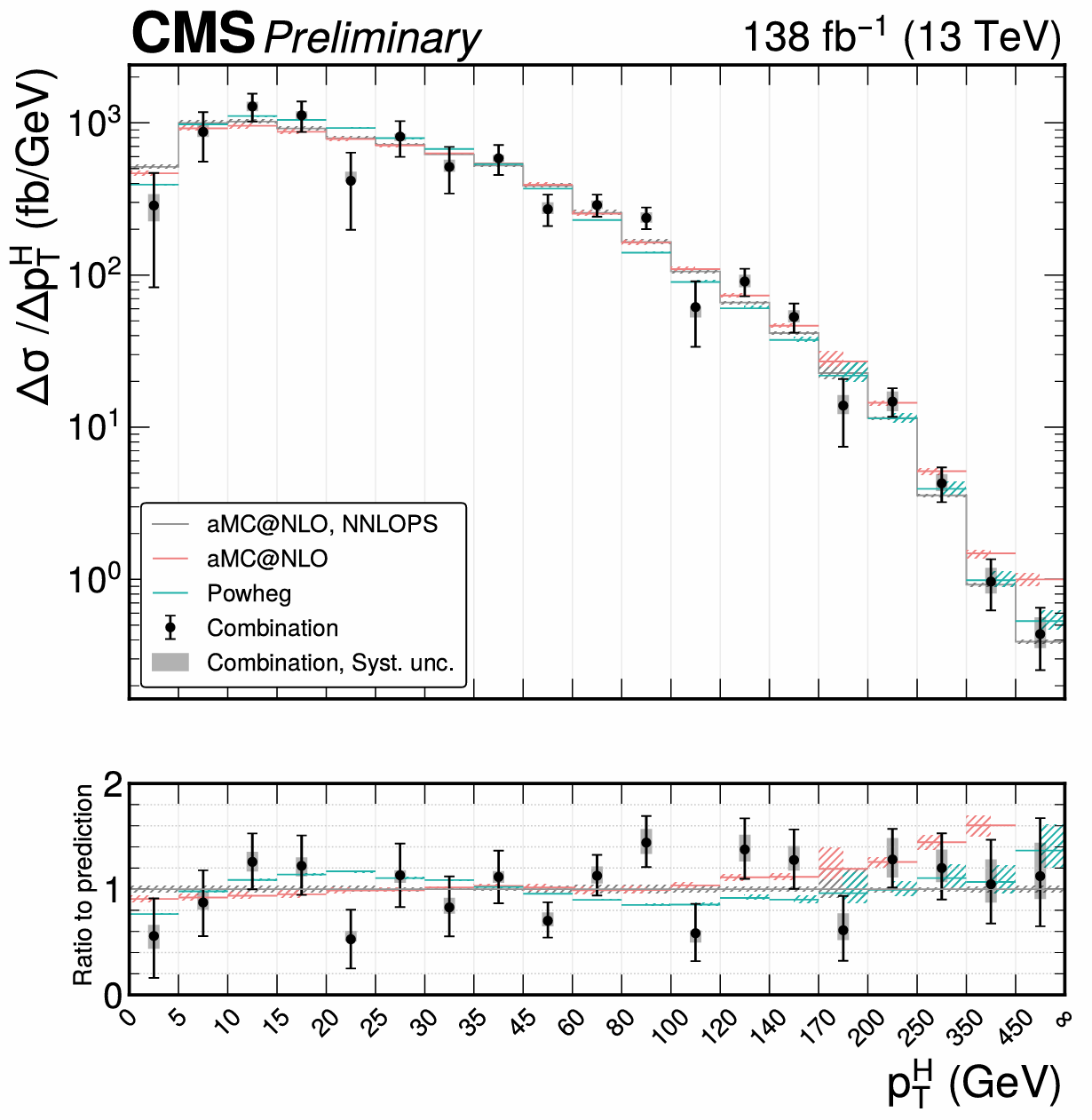
Figure 1: Combined measurement of the rate of production of the Higgs boson in bins of its transverse momentum. The measured values (black markers) agree well with the Standard Model predictions (grey, green and red histograms).
Now, measuring spectra is for sure interesting, but … that’s not all! The shapes obtained can indeed be used to test the validity of the SM and look for hints of physics beyond it. When the couplings between SM particles change even by a small amount, the differential spectra can change drastically. These changes can be parametrized using different theoretical frameworks and the observed data can be used to set constraints on the parameters of the theory. If those parameters are found to be far away from the SM prediction, this could be a hint of new physics!
Two frameworks are used in the recent CMS result: the kappa-framework and effective field theory (EFT) framework.
The kappa framework is the more “simplistic” among the two: it assumes there is a single Higgs boson, with a mass of 125 GeV, and that any possible new physics effects that can be seen in these measurements affect only the couplings between the Higgs boson and other particles. These possible new physics effects are then parameterized in terms of coefficients κ. We used the Higgs boson transverse momentum measurements to set two-dimensional constraints on κc (Higgs boson to charm quark), κb (Higgs boson to bottom quark) and κt (Higgs boson to top quark). An example is shown in Figure 2, where we can see that the results (the black dot indicates the best-fit value) are in very good agreement with what we would expect from the SM (red dot).
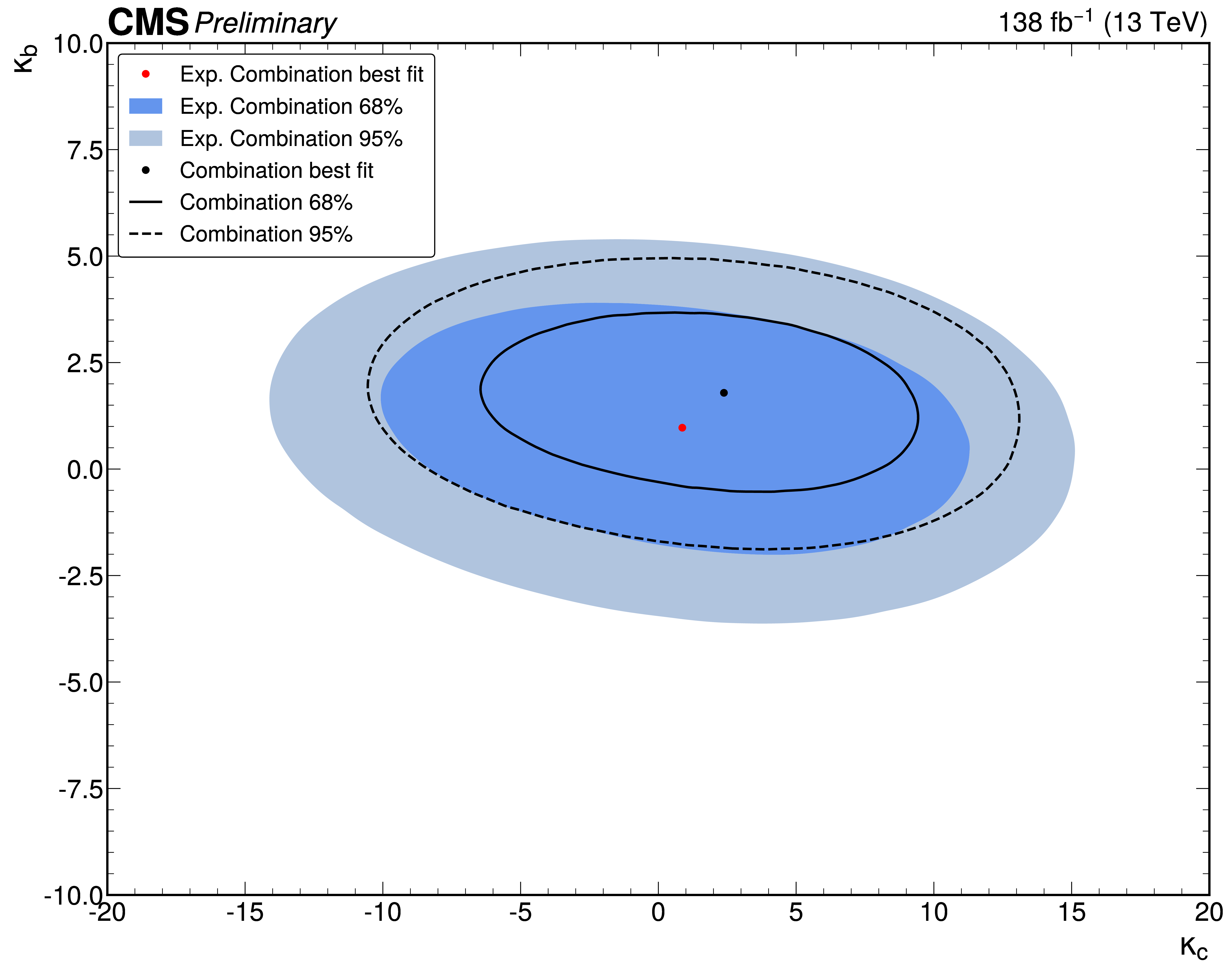
Figure 2: Measured two-dimensional constraints on κc and κb – the black dot indicates the best-fit value – compared with values expected from the Standard Model – the red dot; both sets of values are well in agreement.
Effective field theories (EFT) provide a model-agnostic way to look for possible effects of new physics: the assumption is that these effects happen at an energy scale higher than the one achievable by the current measurements, but their effects at lower energies can be parametrized and studied. EFT introduces new couplings between the SM particles, and each of these couplings comes with a strength governed by a coefficient – which is zero in the SM case since these additional couplings do not exist there. In one of the main parts of this interpretation, we selected a subset of 31 EFT coefficients and fit them one by one while setting the others to their SM value. In all cases, we see that the observed results agree with the SM expectation.
Probing a more general scenario in which all these coefficients are measured together is challenging! Our measurements are not sensitive to all the coefficients in the same way, and trying to constrain one causes degeneracies in others. For this reason, a procedure called “Principal Component Analysis” is applied to select the directions (linear combinations of the coefficients) where the data are more sensitive and fit those instead. This procedure comes from linear algebra and is also used in machine learning to simplify large datasets while maintaining significant patterns and trends. The results are shown in Figure 3, where also in this case, no particular deviations from the SM are detected.
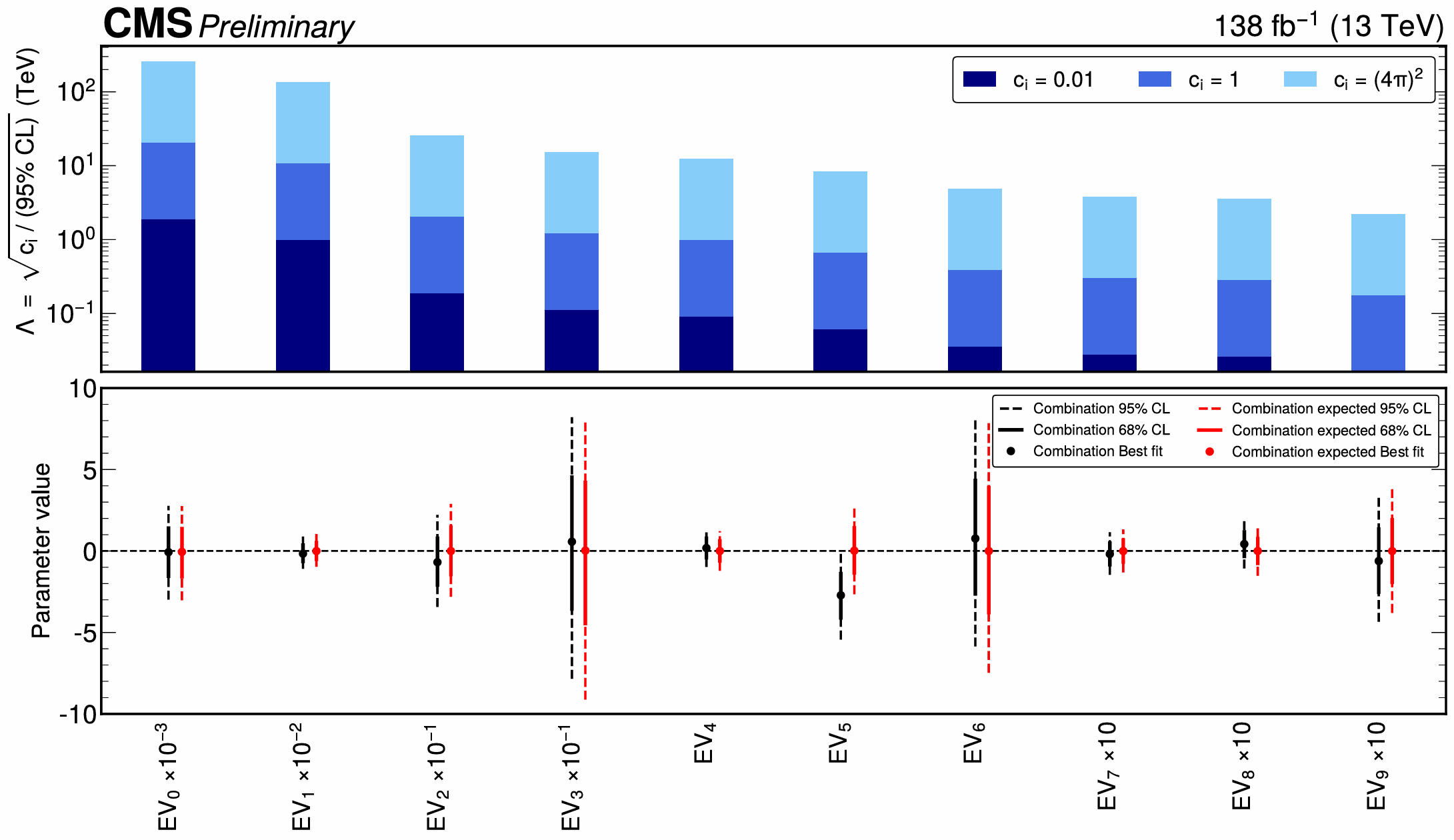
Figure 3: Constraints on linear combinations of EFT coefficients (bottom panel) – the measured values agree well with the SM expectations – and the energy scale of the new physics that they can constrain under certain assumptions (top panel).
Now you might wonder - how can measuring combinations of the original coefficients improve our knowledge about the existence of new physics? These results can be very useful for our colleagues working in the field of theoretical physics: once provided with the definitions of the linear combinations and the constraints derived, they can insert these results in their studies and produce more precise and reliable models of physics beyond the SM for us to test!
Written by: Messimiliano Galli, for the CMS Collaboration
Edited by: Muhammad Ansar Iqbal
Read more about these results:
-
CMS Physics Analysis Summary (HIG-23-013): "Combination and interpretation of fiducial differential Higgs boson production cross sections at 13 TeV"
-
@CMSExperiment on social media: Bluesky - Facebook - Instagram - LinkedIn - TikTok - Twitter/X - YouTube